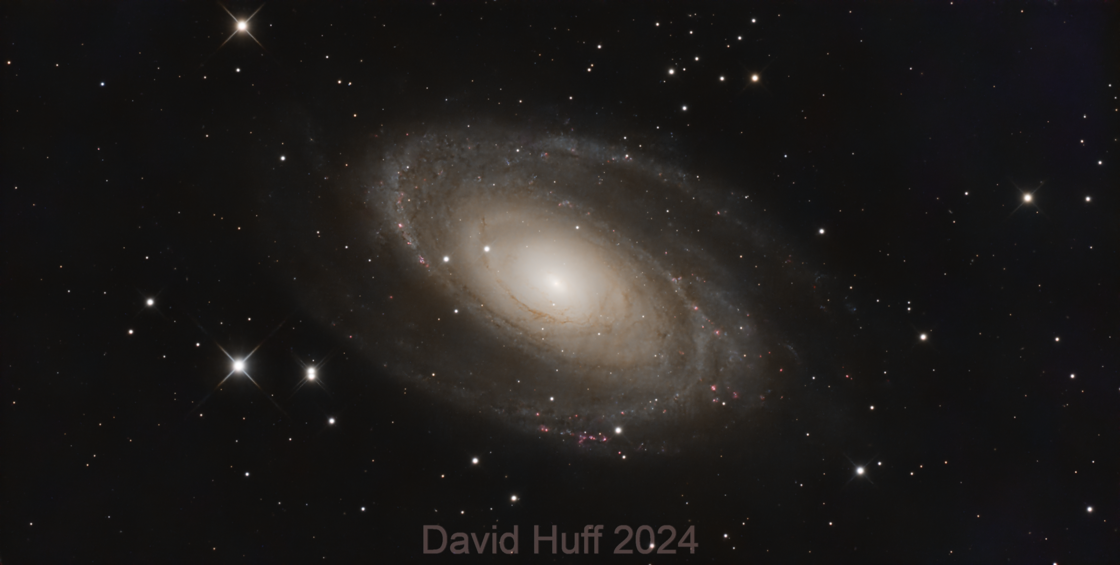
This image is the result of my Fast Imaging project in an attempt to produce my most detailed image of Messier 81 from a light very polluted area. This project began in December of 2023 and though a lot of trial and error, research, and a high electric bill, I finally found the best way to capture and process this subject. Over 80,000 images were taken but only a total of 52,464 sub exposures were kept as I tried from 0.1 second all the way to 30 second exposure times but settled on 21,834 x 1 second and 29,210 x 2 second sub exposures in broadband then 1,420 x 30 second sub exposures using the IDAS NBZ-II filter to capture the faint Ha and apply to the image using continuum subtraction.
See more details like equipment used on my Astrobin: https://www.astrobin.com/q0fzhe/
This was one sub exposure!

Why fast imaging? Glad you asked 🙂. I was never able to image galaxies because they would get lost in the light pollution. This technique seems like it helps a lot! These are my rejection frames from the finished stack and the reason why I used this fast imaging method... Light Pollution! As you can see it does a good job rejecting it! Here is an excellent lecture given by Robin Glover that where I got the idea: https://www.youtube.com/watch?v=3RH93UvP358

These were my image processing steps and settings:
Where I live I have a lot of light pollution and I ended up figuring out a way to analyze and create a Python script that could read the calibrated XISF file and then calculate the the Median Absolute Deviation (MAD) of the subframe data. Then create a report and graph for each run which allowed me remove the outliers that was most likely clouds or excessive light pollution. You can also do this with Subframe Selector and use the median as this can create a graph with similar results.
*** Update: I recently found out that stacking order does not matter for quality with FastIntegration, so you are better off leaving the order and removing any bad frames. I updated the instructions to reflect that.
Graph created by calculating the MAD of subframes to show excessive light pollution.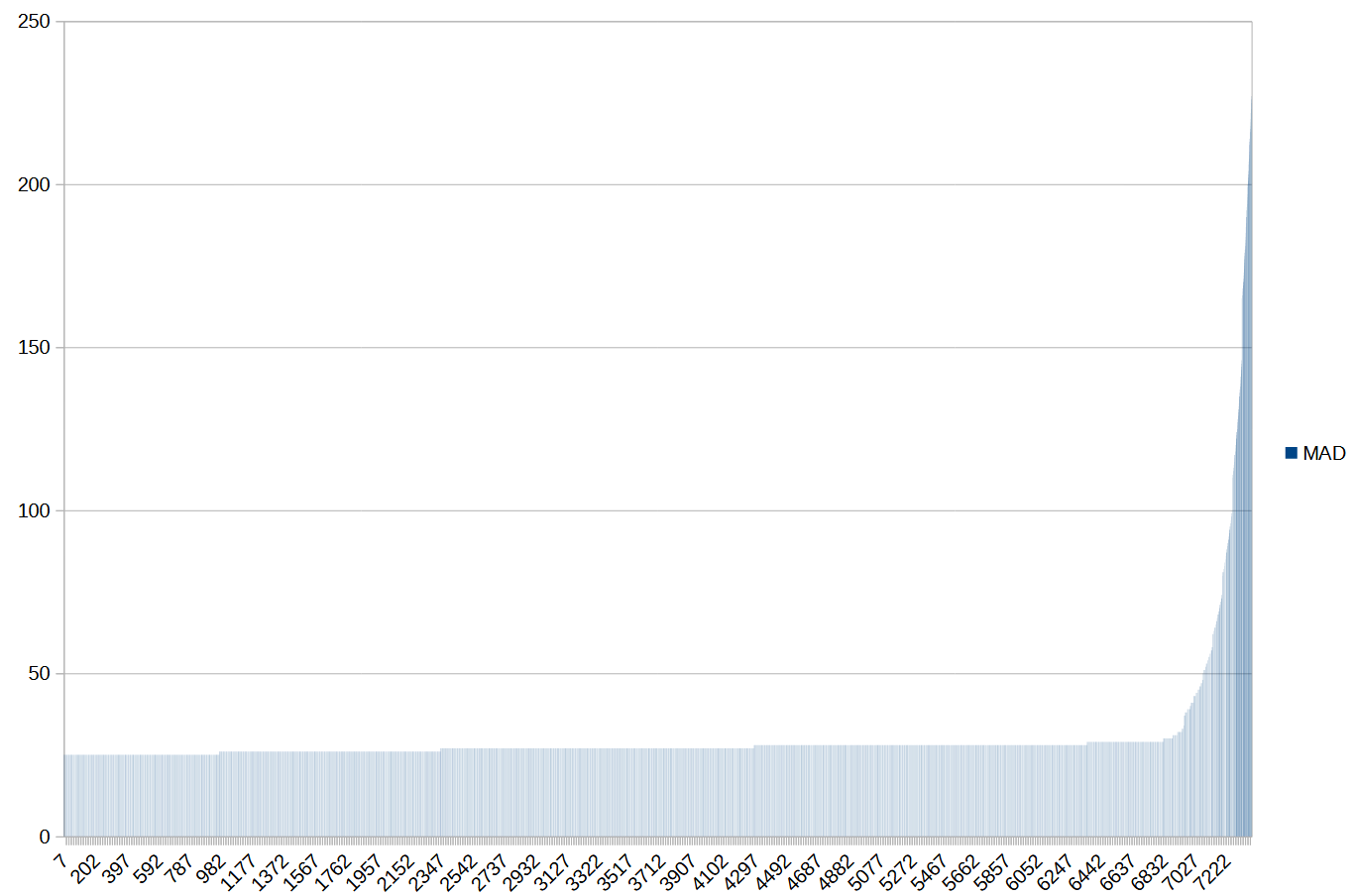
After debayering, I used FastIntegration to create an image with the remaining 52K subframes. I also captured about 1,420 30s dual narrowband sub exposures so I could do a continuum subtraction to add Ha to the image later. For those I just used regular WBPP for best image quality. In the end I decided I would just use the FastIntegration defaults with the exception maxing out the integration and prefetch sizese. Then it would drizzle later to try to remove any interpolation artifacts.
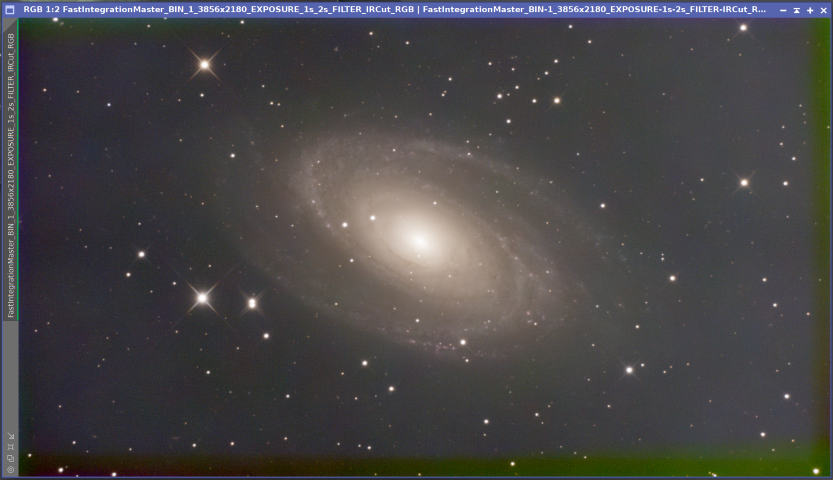
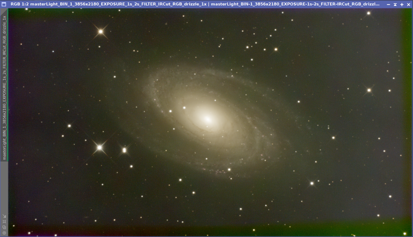
Speaking of drizzle this was another rabbit hole of research but in the end I found that because my data was oversampled, I settled on just using 1x drizzle with a 0.9 drop shrink. This cleaned up the image nicely though it required 15 hours more time, but it was worth the wait! The image below has not been color corrected yet.
Here are the FastIntegration results and drizzle time at the bottom (not sure why the output doubled?):

Processing the resulting image is out of scope of this forum post but I am quite sure that everyone has their own way to make the image beautiful! In the end, I learned a new way to capture images from my even more light polluted location, bad seeing, clouds, and sometimes poor guiding to produce a detailed closeup view of M81 only using a 8 inch Ritchey Criterion telescope!
Clear Skies!
Dave
See more details like equipment used on my Astrobin: https://www.astrobin.com/q0fzhe/
This was one sub exposure!
Why fast imaging? Glad you asked 🙂. I was never able to image galaxies because they would get lost in the light pollution. This technique seems like it helps a lot! These are my rejection frames from the finished stack and the reason why I used this fast imaging method... Light Pollution! As you can see it does a good job rejecting it! Here is an excellent lecture given by Robin Glover that where I got the idea: https://www.youtube.com/watch?v=3RH93UvP358
These were my image processing steps and settings:
- Use WBPP to calibrate darks, flats, and lights (don't debayer yet if OSC). Using darks instead of biases reduce the need for CosmeticCorrection depending on your sensor but add CosmeticCorrection if you still have a lot of hot pixels.
- If using mosaiced images, debayer all of the files into one directory to be used for the FastIntegration process. I used bilinear demosaic for a little speed boost.
- If necessary, use Subframe Selector to analyse and remove frames with lesser quality and excessive background brightness.
- Run the FastIntegration process using the best frame as a reference and the debayered images (calibrated subframes instead if mono, and do one color at a time using the same reference frame for all images) using the default parameters with the exception of selecting create drizzle files and set the integration and prefetch sizes to match your RAM configuration. Also create a fastintegration folder to output the drizzled files using the output directory section.
- Do the DrizzleIntegration process using the drizzle files in the previously created fastintegration folder using the following parameters:
- If using mosaiced data, make sure the check the Enable CFA Drizzle checkbox.
- If using mono data drizzle each color individually and do a channel combination process afterwards.
- For oversampled data, use 1x scale and 0.9 Drop Shrink.
- For well sampled or undersampled data, use 2x scale and 0.9 Drop Shrink.
- Note: You could also experiment with DrizzleIntegration parameters but I found these to be the best for my camera
- Process the resulting image like you normally would
Where I live I have a lot of light pollution and I ended up figuring out a way to analyze and create a Python script that could read the calibrated XISF file and then calculate the the Median Absolute Deviation (MAD) of the subframe data. Then create a report and graph for each run which allowed me remove the outliers that was most likely clouds or excessive light pollution. You can also do this with Subframe Selector and use the median as this can create a graph with similar results.
*** Update: I recently found out that stacking order does not matter for quality with FastIntegration, so you are better off leaving the order and removing any bad frames. I updated the instructions to reflect that.
Graph created by calculating the MAD of subframes to show excessive light pollution.
After debayering, I used FastIntegration to create an image with the remaining 52K subframes. I also captured about 1,420 30s dual narrowband sub exposures so I could do a continuum subtraction to add Ha to the image later. For those I just used regular WBPP for best image quality. In the end I decided I would just use the FastIntegration defaults with the exception maxing out the integration and prefetch sizese. Then it would drizzle later to try to remove any interpolation artifacts.
Speaking of drizzle this was another rabbit hole of research but in the end I found that because my data was oversampled, I settled on just using 1x drizzle with a 0.9 drop shrink. This cleaned up the image nicely though it required 15 hours more time, but it was worth the wait! The image below has not been color corrected yet.
Here are the FastIntegration results and drizzle time at the bottom (not sure why the output doubled?):
Processing the resulting image is out of scope of this forum post but I am quite sure that everyone has their own way to make the image beautiful! In the end, I learned a new way to capture images from my even more light polluted location, bad seeing, clouds, and sometimes poor guiding to produce a detailed closeup view of M81 only using a 8 inch Ritchey Criterion telescope!
Clear Skies!
Dave


